Is It Bias or Noise – Breakout Baseline #6

Ladies and gentlemen… today you’ll see the matchup of a lifetime. All the way from RL Canon, you know it, you love it. It’s entropy bonus!!! If you let them, they’ll make your agent explore from sun up to sun down, never settling on a policy.

In the other corner, a newcomer to the ring, we have Biased Advantage!! They’ve already proven they can produce strong results with Gymnax MinAtar Breakout agents, introducing a correlated exploration signal based on critic certainty. But can they withstand the assault of entropy bonus? Let’s find out tonight! LETS GET READY TO RUMBBLLLEEEE!

Where We Left Off

If you missed the last few posts, here is a quick rundown:

We have been working on getting a baseline PPO agent up and running for the Gymnax MinAtar Breakout environment with the goal of starting a library of baselines for future tests.

While setting up batch-normalized advantage, we stumbled upon a bug that caused a major increase in the real average episodic reward for our agent. An issue but also an opportunity!

So, we went on a quest to uncover why this bug was helping our agent so much. We did a deep dive into our agent’s advantage calculations and, after some digging, came up with a solution that not only fixed the bug but also gave us the same exceptional performance!

We introduced a type of biasing into our advantage estimation. The bias? We’re adding $\displaystyle V(s_0)$ multiplied by some hyperparameter factor to the entire advantage calculation for a given trajectory.

My current theory is that the biasing is beneficial because it causes the agent to explore more when the critic is uncertain about the current value of the environment.

So, today, let’s test out my theory of why this new type of advantage is advantageous (mhmm). If it is true that it’s related to entropy and exploration, we can even compare it to our standard entropy bonus to see which is better.

Go Out And Explore

Okay, so we have two forms of noise we’re adding to our advantage that seem to improve our performance. My working assumption right now is that the reason this biased advantage is so effective is because it results in higher exploration compared to the baseline in states where the critic is less certain.

So our starting hypothesis:

🤔Hypothesis

Using our biased advantage calculation, our agent receives a much higher final average episodic reward because the bias is correlated with the certainty of the critic about the value of a given state, meaning the agent explores more in state where it is uncertain.

This is actually pretty testable. We want to check two things:

Is the biased advantage agent’s entropy generally higher than that of the baseline agent?
Is the biased advantage agent’s entropy generally higher in states when the critic is uncertain?

The first one is quick and easy to check. We’ll just plot the average entropy over time for both our agents and compare the two.

I already have the code for that so I’ll just run the agents and let’s check the results.

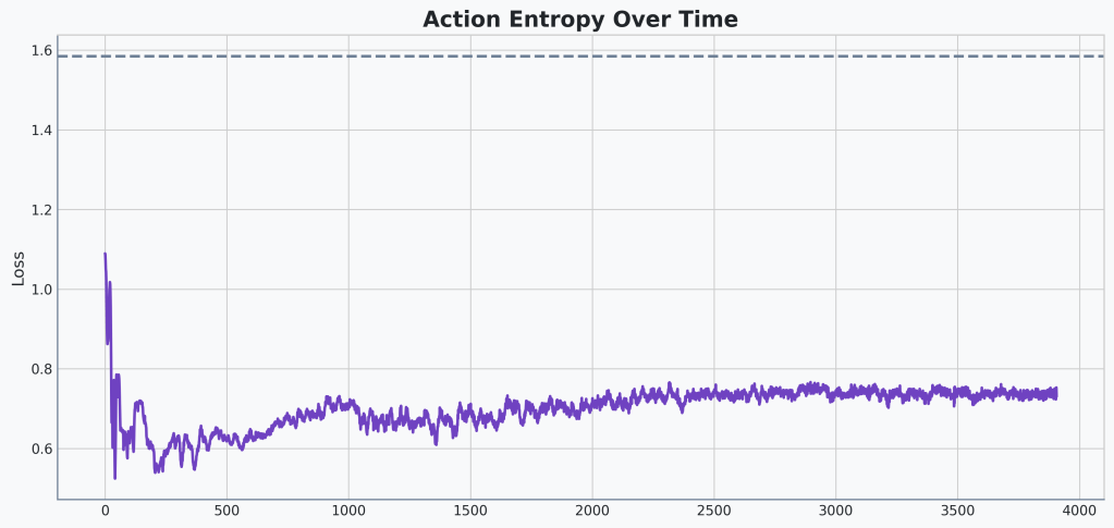
First the base agent:

Versus our biased advantage agent:

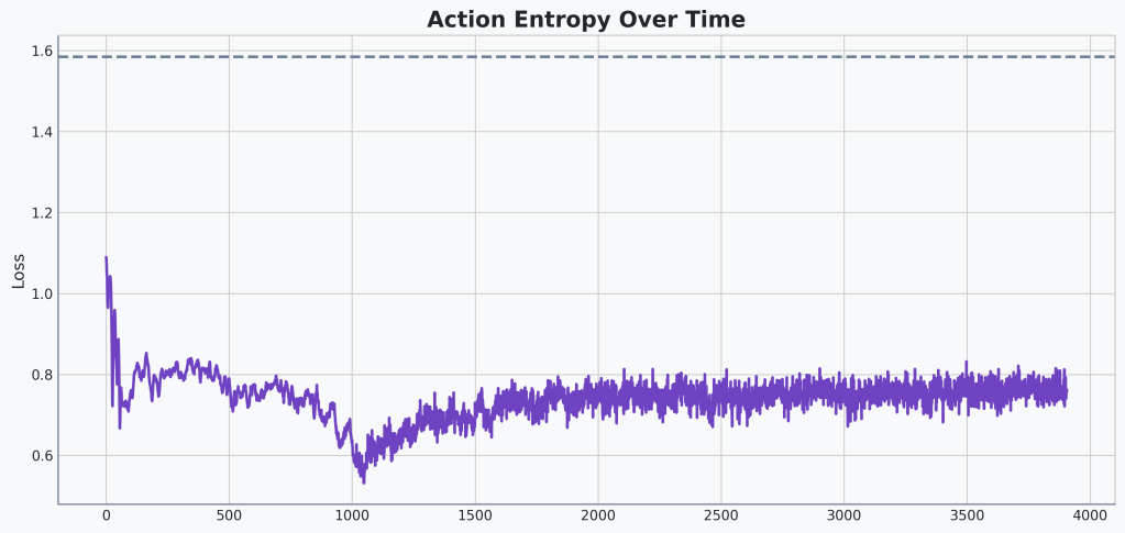
🔍Analysis

Certainly the entropy of our biased advantage agent has higher variance. And except for the spike down at around 1000 updates, the maximum is slightly higher as well.

Well that seems to support our assumptions. Let’s do the more complicated check to see if the entropy scale is correlated to the critic uncertainty.

Doing a quick search for how to estimate uncertainty of a model I came across something called Monte Carlo Dropout. Essentially you run the same critic network multiple times with dropout enabled. Different parts of the network will be dropped in each run. The variance of the final outputs is a good proxy for uncertainty. This seems fit for purpose so let’s code it up! Or, at least I’ll have Gemini do this one for me. It seems like its going to be tedious. And nothing we haven’t done before.

Okay, after some iteration, the code is working. And I’m getting a scatter plot that shows the correlation between the critic variance and the action entropy. Let’s take a look and see if it confirms our suspicions.

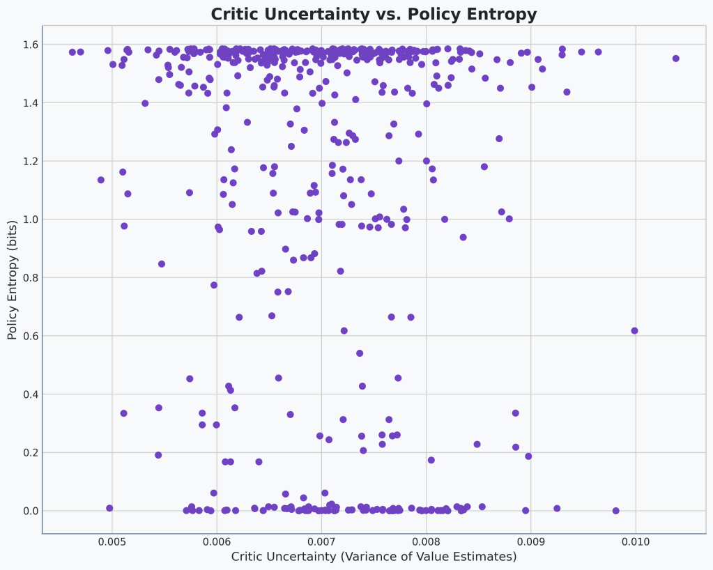
🔍Analysis

Okay. Okay. Okay. I’m not sure I’ve ever seen something so uncorrelated before.

The concentration of points at either maximum or minimum entropy is an interesting artifact to note, though!

So what now? That seems to disprove our hypothesis. We’re back to square one. We have a technique that we know provides a massive performance boost, but we have no idea why. This changes our investigation. The head-to-head comparison with the entropy bonus is no longer a battle between two known exploration strategies. It’s a battle between a known quantity and a mysterious black box.

Back to Square One

If you notice, there are clear bands at the top and bottom of our entropy. The agent seems to be either very certain or very uncertain. But much more rarely is it somewhere in between. Let’s see if the same holds true for our base model.

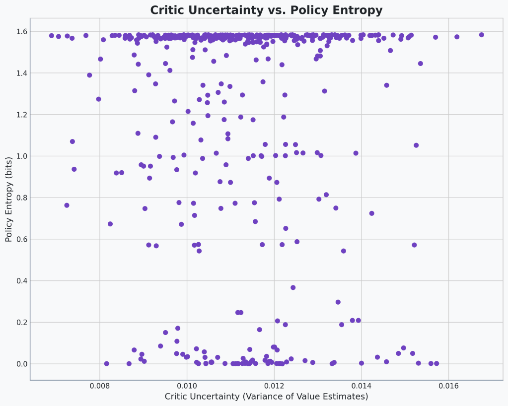
🔍Analysis

Still no correlation, which isn’t surprising. The range of critic uncertainty is higher. That’s also not surprising because the agent performs worse. Otherwise, nothing really to note. This looks basically the same as the previous scatter plot.

Keep It Simple, Stupid

Okay, maybe I’m overthinking this. Let’s do some exploratory visualizations to see if we can see what is going on here. First, I think we can actually just look at the values of $\displaystyle V(s_0)$ that we’re adding to our advantages and see if there’s any interesting correlations there.

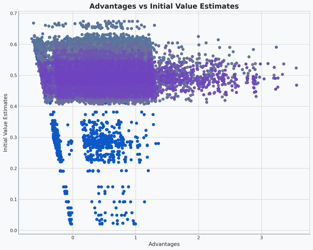
I’ve thrown together a scatter plot that shows a sample of the raw Generalized Advantage Estimation (GAE) that we’ve implemented directly from the PPO paper versus the $\displaystyle V(s_0)$ values we’re adding to them in our biased advantage. I’ve also colored the scatter plot based on how far in to the training the agent is. Blue is early on, gray is in the middle, and purple is at the end. Let’s see if anything stands out:

🔍Analysis

Anyone else see the flag pole?

Okay, a lot to unpack here. The most noticeable thing is that later in the training, the range of advantages is much larger. That makes sense, most of the range is coming from the upper side meaning we’re predicting higher scores, which we’re getting.

The value estimates also seem to drift higher later in training, overshooting a little, and then settling centered around 0.5.

There does also seem to be a bit of correlation here. The whole chart seems to lean to the left.

Okay, why is our chart leaning? I think it’s actually a symptom of our GAE calculation. Let’s take a look at it really quickly.

$\displaystyle \hat{A}_t = \sum_{i=0}^{T-t-i} (\gamma \lambda)^i \delta_{t+i}$

$\displaystyle \delta_t = r_t + \gamma V(s_{t+1}) - V(s_t)$

Notice how, for $\displaystyle \delta_t$ , we’re taking the actual reward and subtracting $\displaystyle V(s_t)$ from it? I think that’s the cause of this slant.

Essentially, if the critic is overly pessimistic, it will predict lower $\displaystyle V(s_t)$ than the actual $\displaystyle r_t$ , meaning we’ll have a higher final $\displaystyle \delta_t$ . As the critic becomes more optimistic, the opposite occurs. $\displaystyle V(s_t)$ will approach and then surpass the actual $\displaystyle r_t$ , meaning we’ll have lower $\displaystyle \delta_t$ values.

So perhaps this is our key! The bias we’re adding to our advantage is correlated with our actual critic’s own bias, whether it is pessimistic or optimistic, about the current value of the trajectory.

Unpacking the Bias

Hmm… in retrospect that seems like a pretty obvious conclusion to come to. Maybe we didn’t need a chart for that.

So, our new hypothesis:

🤔Hypothesis

Using our biased advantage calculation, our agent receives a much higher final average episodic reward because the bias regularizes the critic’s bias. Our biased advantage will be lower when the critic is more optimistic and it will be higher when our critic is more pessimistic.

Again, stating it like that, the mechanism seems pretty obvious. But is that really providing the benefit? Well maybe we can test a different version of advantage that has the same mechanism and see if we get the same boost.

Let’s define a new $\displaystyle \delta_t$ that more highly weights the advantage estimate over the true reward:

$\displaystyle \tilde\delta_t = r_t + \gamma V(s_{t+1}) - (1 + \tau)V(s_t)$

Let’s quickly break down how this new formula works. By multiplying our current value estimate $\displaystyle V(s_t)$ by a factor slightly greater than one, we are effectively increasing its weight in the TD-error calculation.

When the critic is optimistic (predicting a high $\displaystyle V(s_t)$ ), this change makes the subtraction even larger, pushing the final advantage down.
When the critic is pessimistic (predicting a low $\displaystyle V(s_t)$ ), this change has less of a suppressive effect, keeping the advantage relatively higher.

This directly implements our idea of regularizing the critic’s bias in a controlled way. So, if our hypothesis is correct, we should expect to see the same performance boosts we saw with our biased advantage because we’re again regularizing our critic’s bias. Let’s implement it and see how our agent does!

Okay, okay. I got a little too heavy handed with my first $\displaystyle \tau$ value of 0.5 and ran straight into a nan critic loss. Oops. Let’s try again with something a little smaller. How about 0.08, the same value we’ve been using for our biased advantage coefficient.

Okay. Another nan loss. Actually, I have a bug. Let me fix it really quickly. Okay, back on track. Let’s try again!

Model	Avg Episodic Reward	Min Episodic Reward	Max Episodic Reward
Base	9.41	7	12
τ = 0.005	10.84	7	15
τ = 0.01	29.30	13	47
τ = 0.05	16.37	7	25
τ = 0.08	17.77	16	19
τ = 0.2	7.00	7	7

🔍Analysis

There’s a clear increase in performance using our new regularized TD-error calculation! Not the same lift we’re seeing from our biased advantage but we’ve at least got a part of it.

How about that! We see a lift in performance with this $\displaystyle \tau$ -regularization!

That’s got me thinking, though. As I proposed initially, part of the benefit of the biased advantage might just be increased exploration. What if both hypotheses were right? Is the lift partially from this regularization and partially from exploration incentivization?

Back To Noise For the 1000th Time

Since we switched to CNNs a couple posts ago, we haven’t re-tuned our entropy bonus coefficient. How about we turn off all this biasing and normalization and re-tune our entropy bonus to get the best performing model. Let’s see how that compares to our biased advantage. And then let’s add back in our $\displaystyle \tau$ -regularization to see if we can meet or exceed our previous best of 84. Let’s do it!

But first, a quick note. We’re about to see some massive numbers here. I started seeing 84s everywhere. It seems like, somewhere, 84 is a hard maximum even though I don’t see any limits in the code. So that 84 we’re getting from our biased advantage. Maybe not it’s maximum performance.

I don’t think it is a useful comparison if we’re just seeing everything maxing out at 84. So I increased the maximum steps from 1000 to 5000. And then I started hitting the maximum for that too, 417. So I’ve increased the maximum to 10,000. Hopefully that will be enough.

Also, we’re starting to see some pretty big ranges between the min and max returns. I’m going to start including median as well for a better view.

First, our entropy bonus tuning for our CNNs. With this added max steps, runs take forever. See you in a bit…

Entropy Coefficient	Median Episodic Return	Mean Episodic Return	Min Episodic Return	Max Episodic Return
0.05	16	11.68	7	16
0.08	500	503.84	500	508
0.1	606	340.36	52	606

🔍Analysis

We see a huge performance boost with a tiny tweak to our entropy coefficient (and increasing our maximum episode length). We’re seeing rewards up in the 500s and 600s now.

0.1 gets the highest final median episodic reward but also introduces a lot of instability (see the 52 minimum reward). 0.8 is much more stable.

If we keep increasing the coefficient it’s safe to assume this variance will increase.

Okay, so our best performance is 0.08. We could get higher rewards using 0.1 but I don’t like the variance we get in rewards. We weren’t that far off with our previous 0.05. Funny how a little change can make a huge difference.

By the way, I must be getting jaded with this project. Getting 500, compared to the Gymnax GitHub baseline’s 24, doesn’t even phase me.

$\displaystyle \tau$ -Regularization

Speaking of little changes, let’s add our $\displaystyle \tau$ -regularization back in now that we have tuned our entropy bonus and see if we can get even better results.

Our new champion is the agent with a 0.08 entropy bonus. It’s incredibly stable and powerful. Now for the final test: can our novel bias regularization technique improve upon this already stellar performance? Let’s find out.

We’ll keep our entropy coefficient at 0.08 and test a few different $\displaystyle \tau$ values and see how we do. See you on the other side!

$\displaystyle \tau$	Median Episodic Reward	Mean Episodic Reward	Min Episodic Reward	Max Episodic Reward
0.0	500	503.84	500	508
0.005	56	43.53	30	56
0.01	25	412.91	25	834
0.1	821	807.09	792	821
0.2	802	806.79	802	812
0.3	7	7.0	7	7

🔍Analysis

We again see our baseline at the top of the table, which is equivalent to $\displaystyle \tau = 0$ .

We see a pretty big dip in performance starting at low values of $\displaystyle \tau$ .

And then a huge boost in performance at higher ranges of $\displaystyle \tau$ . with the best performers earning final rewards in the 800s.

At the highest end, performance totally degrades.

Wow!! I think we’ve got something here. At small values of $\displaystyle \tau$ we seem to just be introducing some turbulence that is ruining the agents performance but at higher levels, we’re seeing a major increase in performance!

This is really exciting! We’ve gone from having a bug in our code that tricked us into thinking we had an amazing agent (which I guess we kind of did but for the wrong reasons). We then tracked that bug down and fixed it which crashed our performance. But then, through careful evaluation, we’ve come up with a more principled way to get even better results from seemingly the same mechanics. A huge win for the methodical approach. That feels awesome!

But a good researcher is always a little skeptical. Before we pop the champagne, there’s one last question to answer to be absolutely sure we understand what’s going on.

Final Checks

Our theory is that our new $\displaystyle \tau$ -regularization along with the correctly tuned entropy coefficient is a principled replacement for the original ‘helpful bug.’ If that’s true, then re-introducing the original bug should provide no additional benefit.

We should re-introduce our biased advantage to our agent that has the best entropy coefficient and our best $\displaystyle \tau$ . I’m going to go with $\displaystyle \tau=0.2$ because I like that even the minimum episodic reward is in the 800s. If we’ve really captured all the benefit from the original bug, we’ll see either no lift or degradation in performance.

Biased Noise Coefficient	Median Episodic Reward	Mean Episodic Reward	Min Episodic Reward	Max Episodic Reward
0.0	802	806.79	802	812
0.08	673	364.69	30	673
0.1	800	718.01	629	800
0.2	646	640.73	635	646

🔍Analysis

There seems to be no clear benefit to using the biased advantage once both $\displaystyle \tau$ -normalization and entropy bonuses are tuned properly.

The Final Verdict

The results are in. With a median and minimum score of 802, the combination of a well-tuned entropy bonus and our new $\displaystyle \tau$ -regularization is the clear champion.

The End of the Line (For Now)

What a journey this has been. From a starting score of 3.98, through a bug-induced high of 84, and back down to 9, we’ve methodically peeled back the layers of this problem. By refusing to guess and instead focusing on visualization and principled experimentation, we’ve built a final agent that scores a stable ~800, crushing the original baseline.

This, more than any score, is the real victory…

I think, for now, this will be the end of the Breakout Baseline saga. We will likely use the baseline we’ve built here to test new ideas but I think there’s not much benefit staying much longer here to further tune the agent. So, what’s next?

Well, we should see if our fancy new $\displaystyle \tau$ -normalization works for environments besides Breakout, shouldn’t we! So, see you next week when we, hopefully much more rapidly, tune up a baseline for a handful of other environments in MinAtar and test our $\displaystyle \tau$ -normalization in those.

Code

You can find the complete, finalized code for this post on the v1.6 Release on GitHub

The Principled Agent