The Principled Agent

The case landed on my desk late. The loss curves were a mess, all volatility and noise, the kind of data that spells trouble. Then the score walked in: 84. A perfect score. Too perfect.

I’d been chasing that number for days. Turns out, the whole thing was built on a lie: a bug in the advantage calculation, whispering sweet nothings in my agent’s ear. I squashed it, and the score didn’t just drop, it cratered. Back to a measly 9. A real slap in the face.

The case wasn’t closed. It had just begun. The real mystery wasn’t why my agent was failing now, but why a bug had made it look so good. It was time to investigate.

Where We Left Off

Okay, okay. Enough with the noir detective stuff. If you missed the last post, here is a quick rundown:

We’ve been working on a baseline agent for Gymnax’s Minatar Breakout environment using an actor-critic PPO implementation. The goal of which is to start a library of baselines I can test different ideas with.

Last time, we switched the agent from MLPs to CNNs to better suite the environment data we’re getting for Breakout. We then started investigating how to properly tune the CNN hyperparameters (which I hope to eventually get back to) before uncovering an issue with our advantage scaling in our policy loss.

Applying a standard technique in PPO where we batch-normalized our advantage, we saw a huge jump in average episodic reward up to 84 compared with the Gymnax baseline of 28. We celebrated!

And then we found a bug. When we fixed the bug, our performance dropped all the way from 84 down to 9.41. Dang!

The bug basically meant we were calculating advantages wrong. The observation we use to calculate our returns for what should have been the final observation in the rollout was actual the first observation. So we were starting the whole calculation with an incorrect reward! This means the entire advantage signal my agent was learning from was based on a state it wasn’t even in. The ‘good’ performance wasn’t fake but it was based on nonsensical data.

So that’s where we left off. We have a bug that gives us really good performance and it’s unclear why. Today, we’re going to figure out why so we can reproduce our great results in a more principled way.

Twinsies!

First things first. Let’s get a feel for how or bugged advantage looks compared to our correct advantage. Let’s make a graph of the two side by side. It was pretty easy to throw together a chart that plots the min and max batch advantages over time. I was also originally plotting the mean, but of course that is always 0; we’re normalizing by it!

First let’s check out the correct advantages:

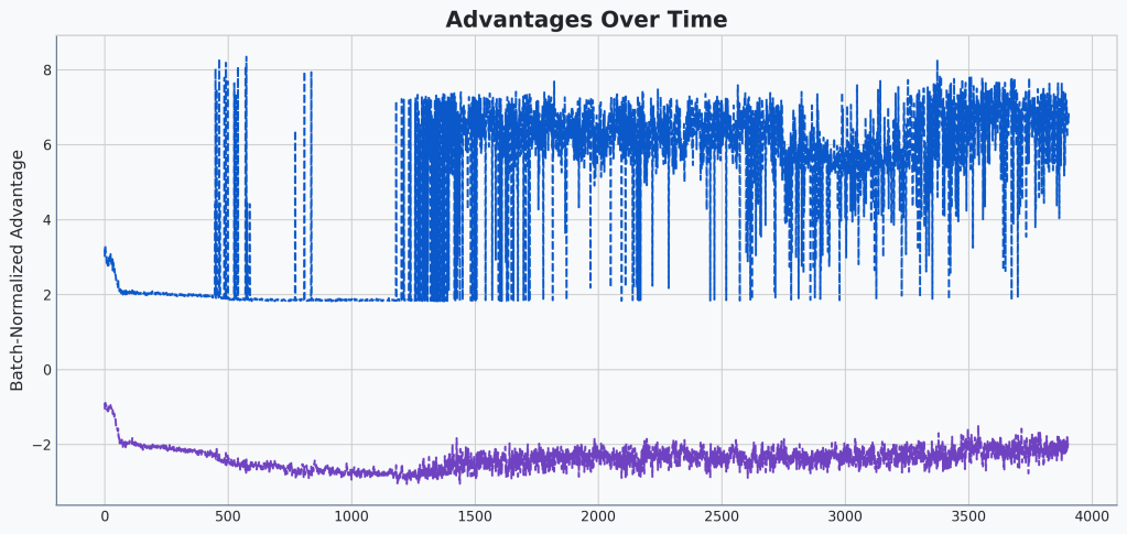
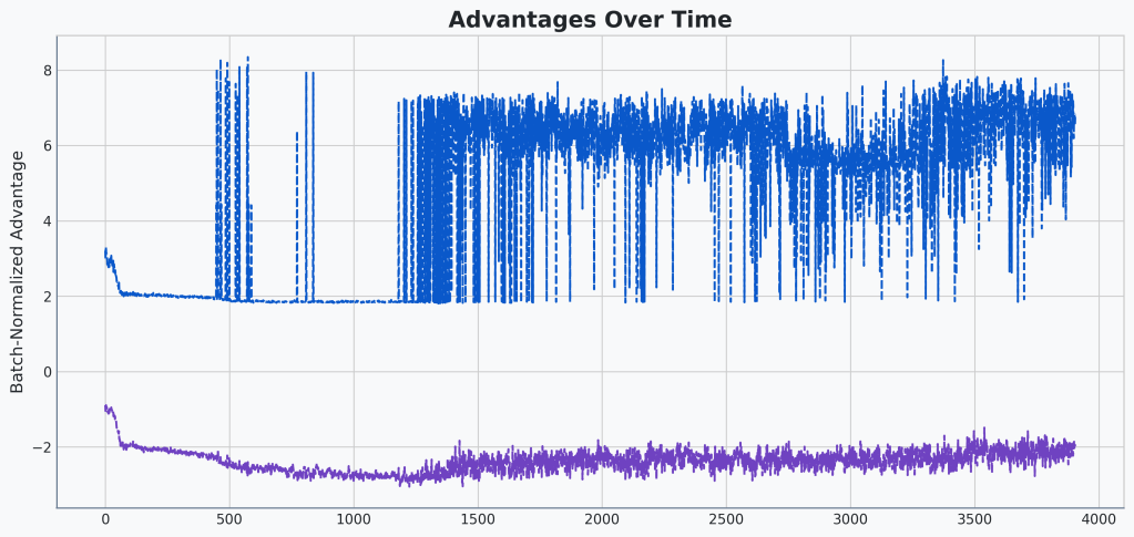
Okay, and the buggy advantages:

Turns out that isn’t very helpful. They look identical. There’s two things I think might be happening here. The first option is that they could be slightly different but at this scale it is hard to tell. The second is that min and max are too crude of metrics to capture the difference.

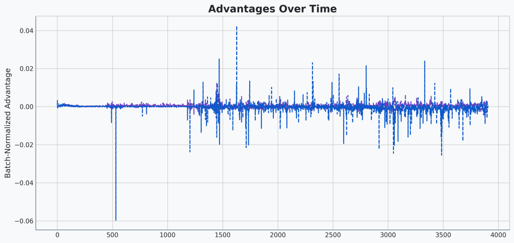
The first is easier to verify so let’s check that first. I’ll plot the difference between the two. That should show us some clear differentiation if there is any. Specifically, I’ll graph the correct advantages minus the buggy advantages. Let’s take a look:

So there are differences. I’m not going crazy. The differences look noisy to me, though it’s hard to tell what the underlying dynamics of the environment are when we see different jumps. Seems like most of the difference is in the higher side of the advantages and that the buggy advantages are being over-estimated.

Well, one simple explanation for the data is that the bug was essentially adding unpredictable noise to the advantage signal, particularly for high-reward actions. Why would this help? My theory is that this noise acts as a form of unstructured exploration. When the agent identifies a good move, the buggy advantage sometimes shouts ‘This is the best move ever!’ and other times just says ‘Eh, it’s pretty good.’ This inconsistency could prevent the policy from converging too quickly and greedily on a single strategy, forcing it to maintain a slightly more open mind. Let’s turn that into a testable hypothesis!

Noisy Batch-Normalized Advantage

Okay. That’s an easy enough hypothesis to test. Let’s just add some random noise to our advantages and see if it improves performance. The scale will be essential so I’m going to aim for something that matches what we’re seeing in our difference graph above.

So, specifically, I’m adding Gaussian noise to my advantages after they’ve been batch-normalized. The noise standard deviation is 0.005.

Let’s run it and see what happens!

Model	Avg Episodic Reward	Min Episodic Reward	Max Episodic Reward
Baseline	9.41	7	12
Baseline + Random Noise (0.005)	19.49	7	31

Awesome! That actually helped our model’s performance quite a bit! This seems to support our hypothesis. But, just like when we were looking at our entropy bonus, though, we’re seeing a much higher variance in our episodic rewards.

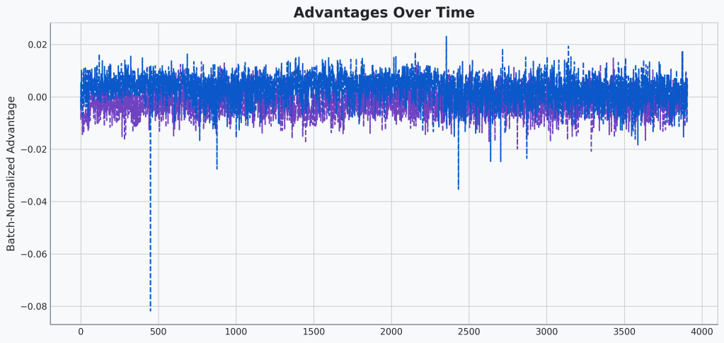
Let’s take a quick look at our advantages difference chart to see if we hit our noise target:

Let’s cut that standard deviation down from 0.005 to 0.0005 and see if we can’t hone this in, get higher rewards, and reduce that variance we’re seeing in our episodic rewards.

Model	Avg Episodic Reward	Min Episodic Reward	Max Episodic Reward
Baseline	9.41	7	12
Baseline + Random Noise (0.0005)	7.52	7	8
Baseline + Random Noise (0.005)	19.49	7	31

Okay, either I overshot or less noise is the wrong direction. Two more tests to see which it is. 0.001 and 0.01. Be back when they’re done running.

Model	Avg Episodic Reward	Min Episodic Reward	Max Episodic Reward
Baseline	9.41	7	12
Baseline + Random Noise (0.0005)	7.52	7	8
Baseline + Random Noise (0.001)	58.04	57	59
Baseline + Random Noise (0.0025)	57.96	57	59
Baseline + Random Noise (0.005)	19.49	7	31
Baseline + Random Noise (0.01)	23.68	19	28

Wow! A major boost in performance. We’re back up above the Gymnax GitHub baseline of 28 up to 58.04 at our highest! This time without any bugs (I hope)! More data to support our hypothesis.

Okay, so what’s happening here. I believe that by injecting noise into the learning process, we’re improving exploration. This means our agent isn’t getting stuck in it some suboptimal policy and is instead motivated to explore outside of it.

“Hold on a second,” you might be saying, “isn’t that what the entropy bonus is for?!”

Well, yes, indeed it is. And this wouldn’t a principled analysis if I didn’t compare this new advantage noise to standard entropy bonuses. But before we get there, I had one other idea.

The Serendipitous Signal

The noise we’re adding in the previous section is completely uncorrelated. The noise from our original bug has two ways it is correlated:

1. The noise is exactly the same across a single trajectory
2. The noise is tied to the uncertainty of the critic’s prediction

Okay, what do I mean. First of all, with the bug, the whole trajectory gets a single noise value based on the first observation in that trajectory. So, essentially, for each trajectory, the critic decides whether this is an “optimistic” or “pessimistic” trajectory based entirely on how it feels about the first state in the trajectory.

Second, if a critic is uncertain about a state, it produces high variance predictions, resulting in higher variance in our noise predictions. Essentially, the more uncertain our critic is, the more exploration it will produce. As it becomes more certain, the exploration will naturally decrease.

That second mechanism sounds really appealing. Let’s actually intentionally add this back in, this time systematically, and see if it improves our score. So a hypothesis:

First, let’s keep our correct advantage calculation the way it is. But now, instead of adding random noise, we’ll add in our critic’s value estimation of the first observation again across the whole set of advantages from a single trajectory. And then we’ll batch-normalize the advantage.

Let’s call this Biased Batch-Normalized Advantage.

I am also going to introduce a coefficient to control how strongly we apply this biasing term. Right now, we are using trajectories of length 256 with a discounting gamma of .95. Using the sum of a finite geometric series, we can calculate what our average bias across our entire trajectory was while we had our bug.

So we’ll try some coefficients around . Let’s take a look!

Model	Avg Episodic Reward	Min Episodic Reward	Max Episodic Reward
Baseline	9.41	7	12
Baseline + Random Noise (0.001)	58.04	57	59
Baseline + Correlated Noise (0.01)	9.41	7	12
Baseline + Correlated Noise (0.08)	84	84	84
Baseline + Correlated Noise (0.5)	20.03	7	34
Baseline + Correlated Noise (1.0)	55.53	29	84
Baseline + Correlated Noise (1.5)	17.13	7	28

Wohooo! Those data seem to support our new hypothesis. We’re seeing a definite improvement even over the random noise we were using previously. We’re back up at 84! This seems like a very powerful bias to add to the pre-normalized advantage.

Let’s see if we can make that a stronger claim next time.

The Final Word

What a result! We’ve successfully reverse-engineered our “helpful bug” and found a powerful, if unconventional, way to boost our agent’s performance back to a stellar score of 84.

But this discovery raises two critical questions:

1. Is this just a convoluted way of encouraging exploration? Can we achieve the same score by simply tuning the standard entropy bonus?
2. If this new “correlated noise” technique is so effective, could it make the entropy bonus obsolete?

Answering these is the key to knowing if we’ve found a genuinely new trick or just a different path to the same destination. And that’s exactly what we’ll investigate next time.

Code

You can find the complete, finalized code for this post on the v1.5 Release on GitHub.